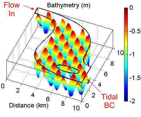
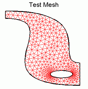
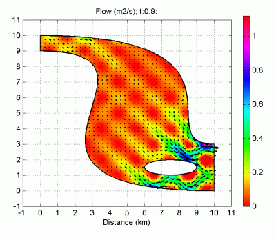
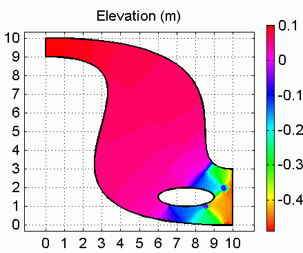
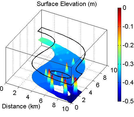
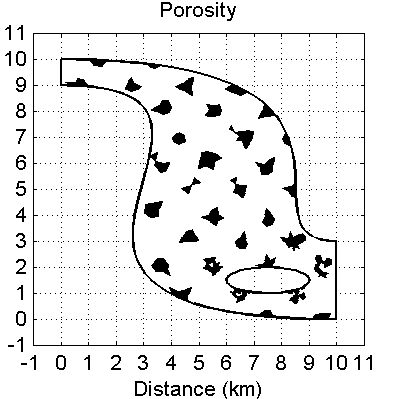
For the test case, we use the geometry and bathymetry illustrated on the right. Since a source of strong non-linearities is the estuarine bathymetry, we use a Sin(x)Cos(y) generated surface for the test case. A constant flow in is specified at the upper boundary, while a 2 m sinusoidal tide (± 1 m) with a 12.42 h period drives the lower boundary. All other boundarys are specified as zero normal flow (i.e., slip BC).

Flow Field.

This movie (click image) shows the flow field (m2/s) for one tidal cycle. Flow can be seen between the "cones" introduced by the SinCos bathymetry model. The tops of some of the cones become dryied as the tide drops below zero elevation.

This simulation (click image) shows water surface elevation during one tidal cycle. Drying of "cones" nearest tidal mouth is evident.

This simulation shows a transient when the tidal boundary is set to -0.5 m and left there at time zero. In effect, the estuary beings to drain out, exposing the high points in the bathymetry. Note that water gets retained in the exposed cones due to the slow transport associated with groundwater model with respect to the open water equations.

This is the same simulation as above, except black spots illustrate where the water surface is below the surface of the bathymetry. That is, the ground water equations dictate the flow in these locations. The irregular shapes of the dried surfaces are caused by the relatively course FE mesh used (see above).