In order to study the impact of organic matter and nutrient loading on food web dynamics, a 1-D, tidally averaged, advection-dispersion model was developed. The governing equation of this model is given by
where
The dispersion coefficient as a function of location and river discharge has been estimated in the Parker River-Plum Island Sound Estuary, MA, from both dye studies and salinity transects. In the dye study, an inert dye (rodamine WT) was released in the upper Parker River, and its concentration profile was measured with a fluorometer at several subsequent high tides. Parameters in a function used to model the dispersion coefficient were then adjusted so that the dye distribution was accurately reproduced by the advection-dispersion model. This is illustrated by this figure, in which measured dye profiles (shown in open symbols) are compared to model output in sold lines for tidal cycles 1, 3, and 5.
Under steady state conditions, the dispersion coefficient can be estimated from the following equation
where C(t,x) is the concentration of an inert tracer (i.e. salt) and q(t) is volumetric flow rate. Consequently, the dispersion coefficient can be estimated from salinity profiles. From salinity profiles during different river discharge regimes, we have obtained the following equation to describe dispersion (m2 s-1) in the Plum Island Estuary (see figure)
where x is distance (m), and q is volumetric flow rate (m2s-1)
Cross sectional river area for the Parker River was measured and fit to the following simple function
The food web model is based on the following diagram
which consistes of autotrophs, heterotrophs, dissolved inorganic nitrogen (DIN), and dissolved organic matter (OM) that is represented in both labile and refractory pools. The heterotrophs are able to graze the autotrophs as well as utilize the DIN and labile OM pools and mineralize organic nitrogen. The food web is an example of a "lumped" model, in that the heterotroph pool consists of organisms ranging in size and taxon from bacteria to macrozooplankton. The autotroph pool is similarly represented.
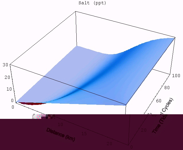
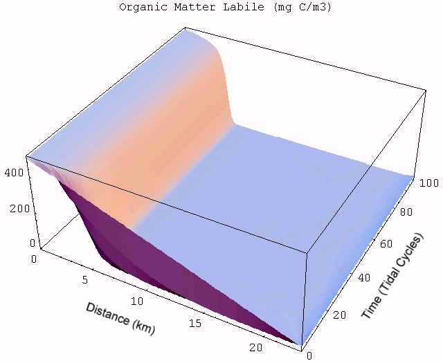
| An animated simulation of the model output showing the transient start-up of the food web from initial conditions can be viewed by clicking the figure on the right. The simulation illustrates the dynamics of autotrophs (Auto) being grazed by heterotrophs (Hetero) along the length of the estuary (distance in km) starting from the head of the river to the ocean. Changes in DIN and labile OM are due to both the biotic reactions and mixing with the ocean. Pure mixing is best illustrated by the monotonic increase in salinity (Salt), which behaves as a conservative tracer in estuaries. | 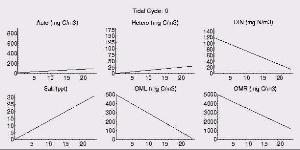
|
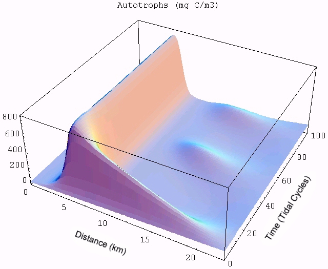
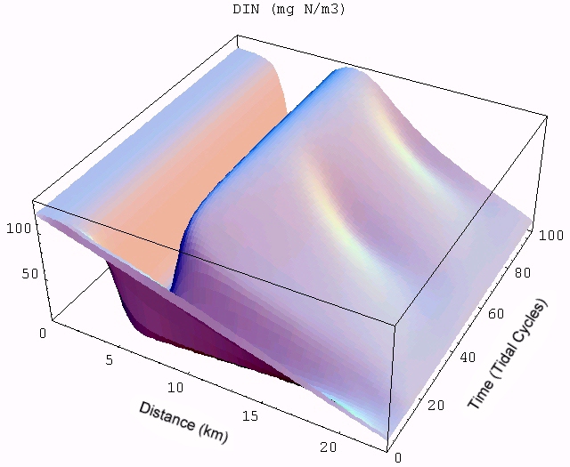
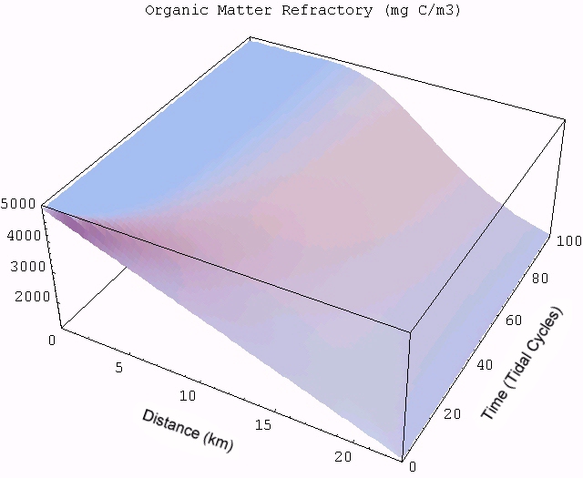
The transient for the autotrophs last about 1 wk (1 tidal cycle equals 12.25 hr), while that for the heterotrophs last about 2 wks. However, predator-prey oscillations are evident in the down stream portion of the estuary. The labile organic matter comes to approximate steady state in only 2 d. Static, 3D images of the state variables versus time (tidal cycles) and distance (km) can also be examined by clicking the thumbnail figures below. Figures were rendered in Mathematica.
| Autotrophs | Heterotrophs | DIN |
 |
 |
 |
| Salt | OM labile | OM Refractory |
 |
 |
 |
A variation of this model was used to examine the autotrophic-heterotrophic nature of estuaries. See Hopkinson and Vallino (1995) Estuaries, 18: 598-621. Also see Vallino, J.J. and Hopkinson, C.S. (1998). Estimation of Dispersion and Characteristic Mixing Times in Plum Island Sound Estuary. Estuarine, Coastal and Shelf Science 46, 333-350.
Code used to solved the above problem is written in Fortran, and the algorithm employed to solve the 1D PDE is a moving-grid method developed and written by Blom and Zegeling (1994), ACM TOMS 20: 194-214. (TOMS731).
Steady state solutions have also been obtained using a collocation algorithm to solve the resulting boundary value problem (COLNEW: Bader and Ascher (1987), SIAM J. Sci. Stat. Comp. 8: 483-500).
Although not used in this particular project, we have found the BACOLR routine to be very efficient at solving 1D ADV equations (R. Wang, P. Keast, and P. H. Muir. Algorithm 874: BACOLR-spatial and temporal error control software for PDEs based on high-order adaptive collocation. ACM Trans.Math.Softw. 34 (3):1-28, 2008.)
All code is available here; however, there is no documentation.